


Chapter Contents
Credits: Benjamin Brown-Steiner
Updates: Page last updated on April 12, 2024
Image above: The sea level change “mug-model” available from the PRI website (accessed April 2024). This mug presents a possible sea level rise scenario when hot liquid is added. The left image shows a present-day scenario while the right image shows an extreme future scenario.
There is a mug that you can buy through the PRI website that changes its appearance when you add hot liquid. This mug shows a map of the world and will show current ocean levels when cold, and a sea level map of some future scenario when hot. While this is a nifty interactive demonstration of global sea level rise scenarios, upon closer inspection there are two major takeaways:
First, this mug – under almost any definition – is a climate model. It is a climate “mug-model.”
Second, it is not a very good climate model.
To the first point: the mug represents, just as climate models represent, a possible change in a potential future climate. The mug represents our planet with both a “present day” and a “potential future” and uses simple principles of physics to simulate what a changed climate would look like. It represents an initial condition (the present-day “cold” map) and, given a command to run (in this case, hot liquid) provides an output (namely a map of future global sea levels).
To the second point, this mug-model is a substantial – almost insulting – oversimplification of a very complex process filled with uncertainties. The mug-model’s parameters cannot be changed or inspected, the input data is locked in, there is only one extreme sea level scenario available, the only output the mug-model provides is a single low-resolution map of sea level, and it doesn’t include any references!
This (albeit somewhat silly) examination of the mug-model provides a decent representation of what a climate model actually does, and what it takes to develop a trustworthy climate model. The necessary components of a climate model include:
- A representation of our best understanding of how the climate system (see Figure 1) works (science, math, and code)
- Input data (initial and boundary conditions)
- Output data (large files filled with numbers that can be interpreted after a model run is finished)
- Tuning or adjustment knobs (parameters and parametrizations)
- A trustworthiness assessment (uncertainty quantification and validation/verification)
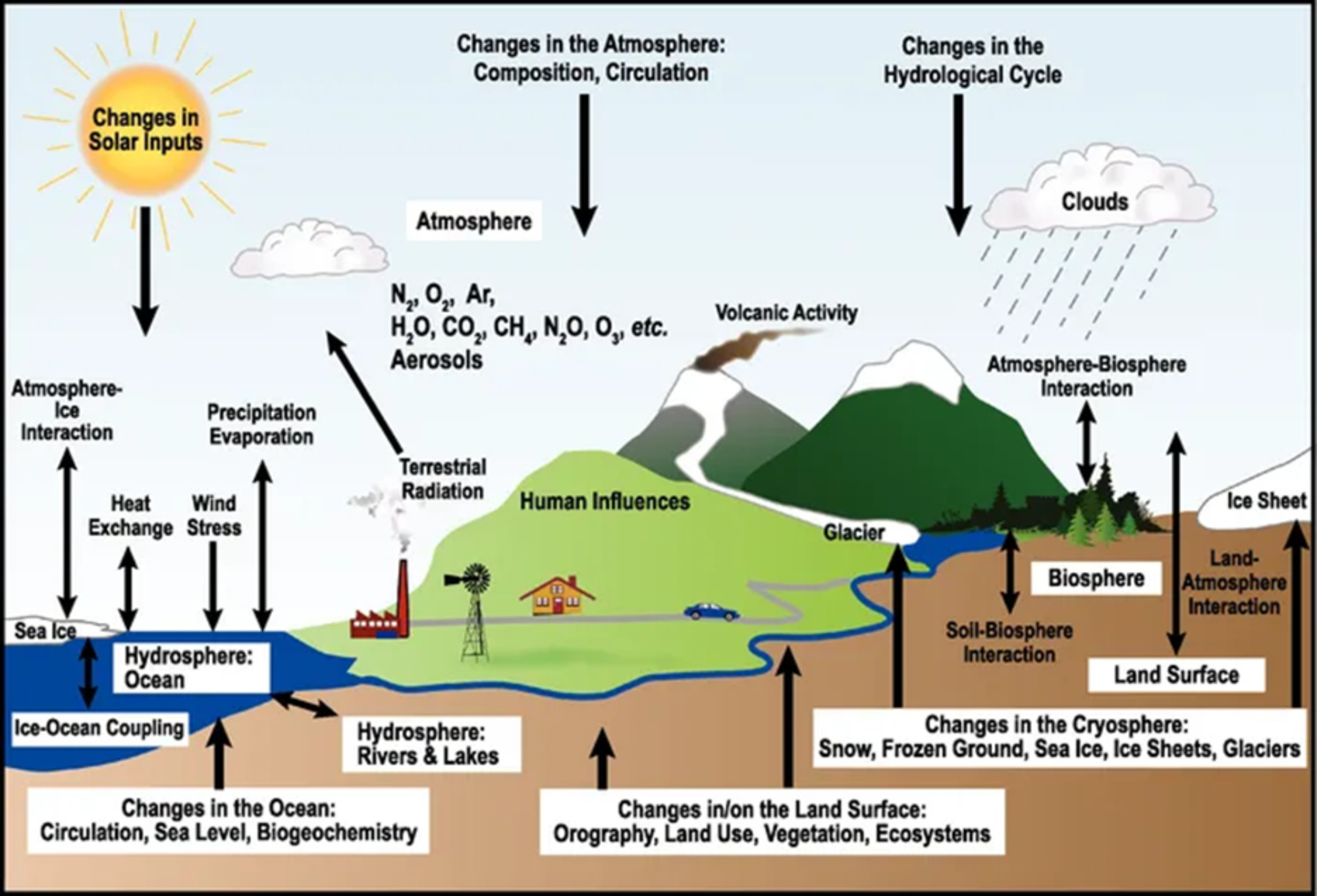
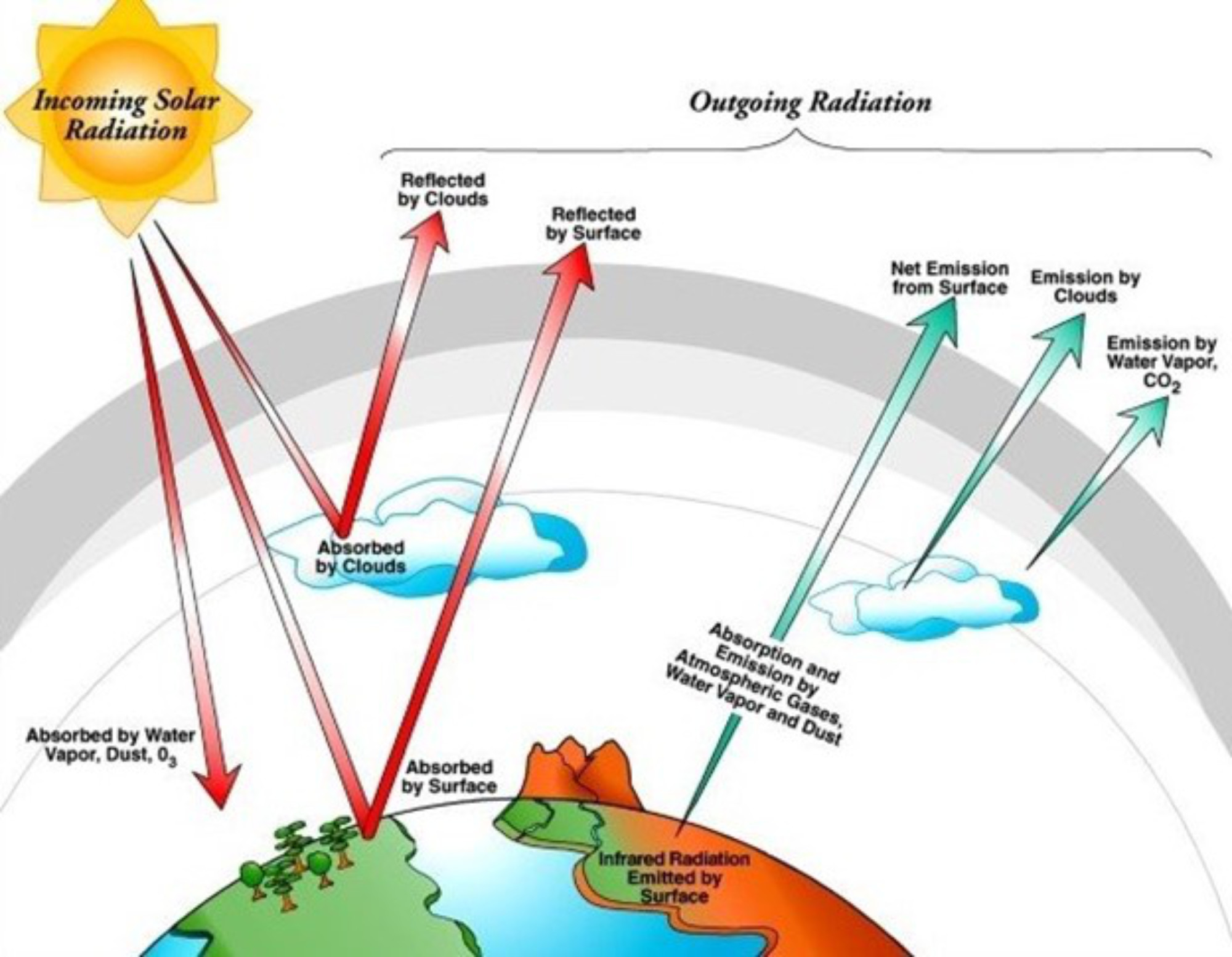
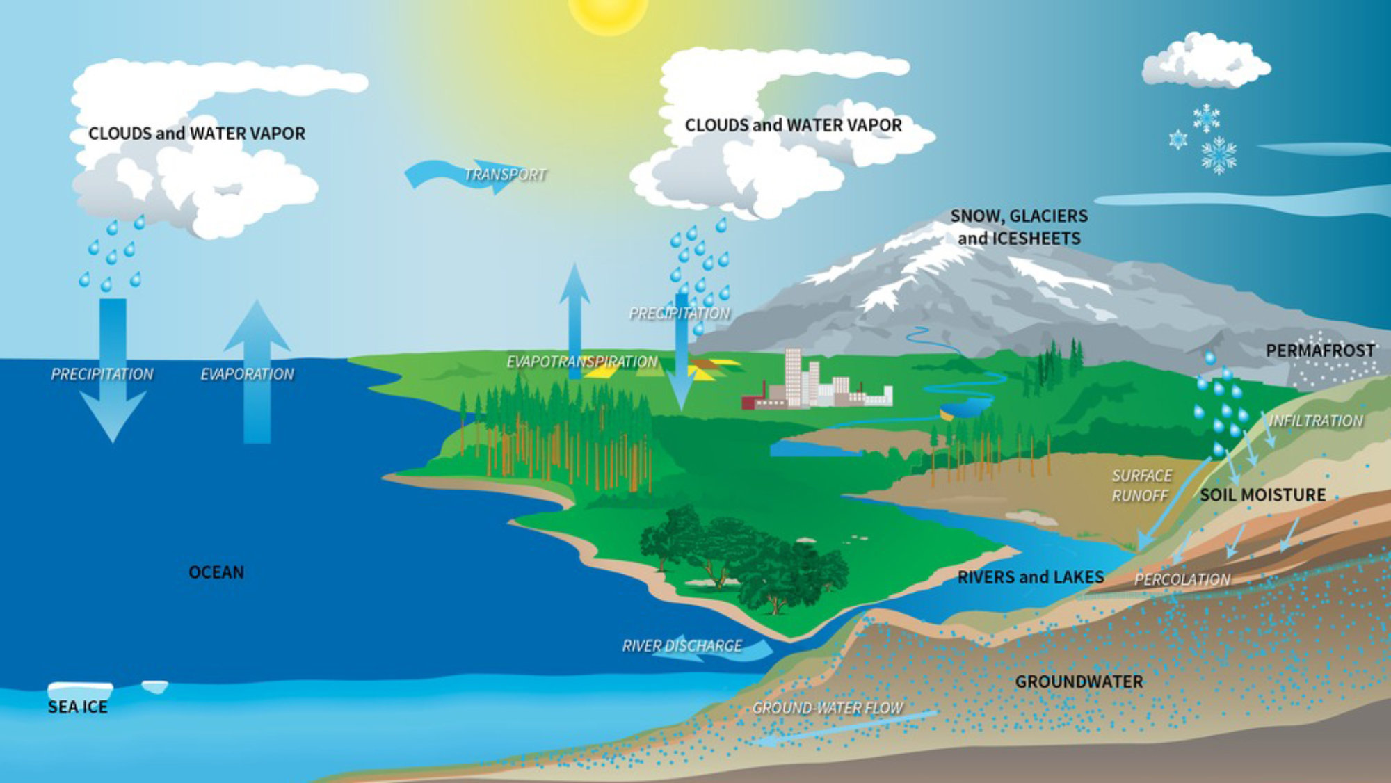
Figure 1: A schematic representation of the climate system highlighting specific systems (including the atmosphere, hydrosphere, geosphere, biosphere, cryosphere, and the sun) and their interactions. Image from UCAR Center for Science Education.
Let’s take a close look at these individual components.
Science, Math, and Code
These three components are the backbone of all climate models upon which everything else relies. And while, like all software, the fundamental pieces are made up of zeros and ones, different models are written in different programming languages. Since most climate models were originally written in the 1950s, 1960s, and 1970s, they used the most reliable and stable coding language of the time – FORTRAN (Figure 2).

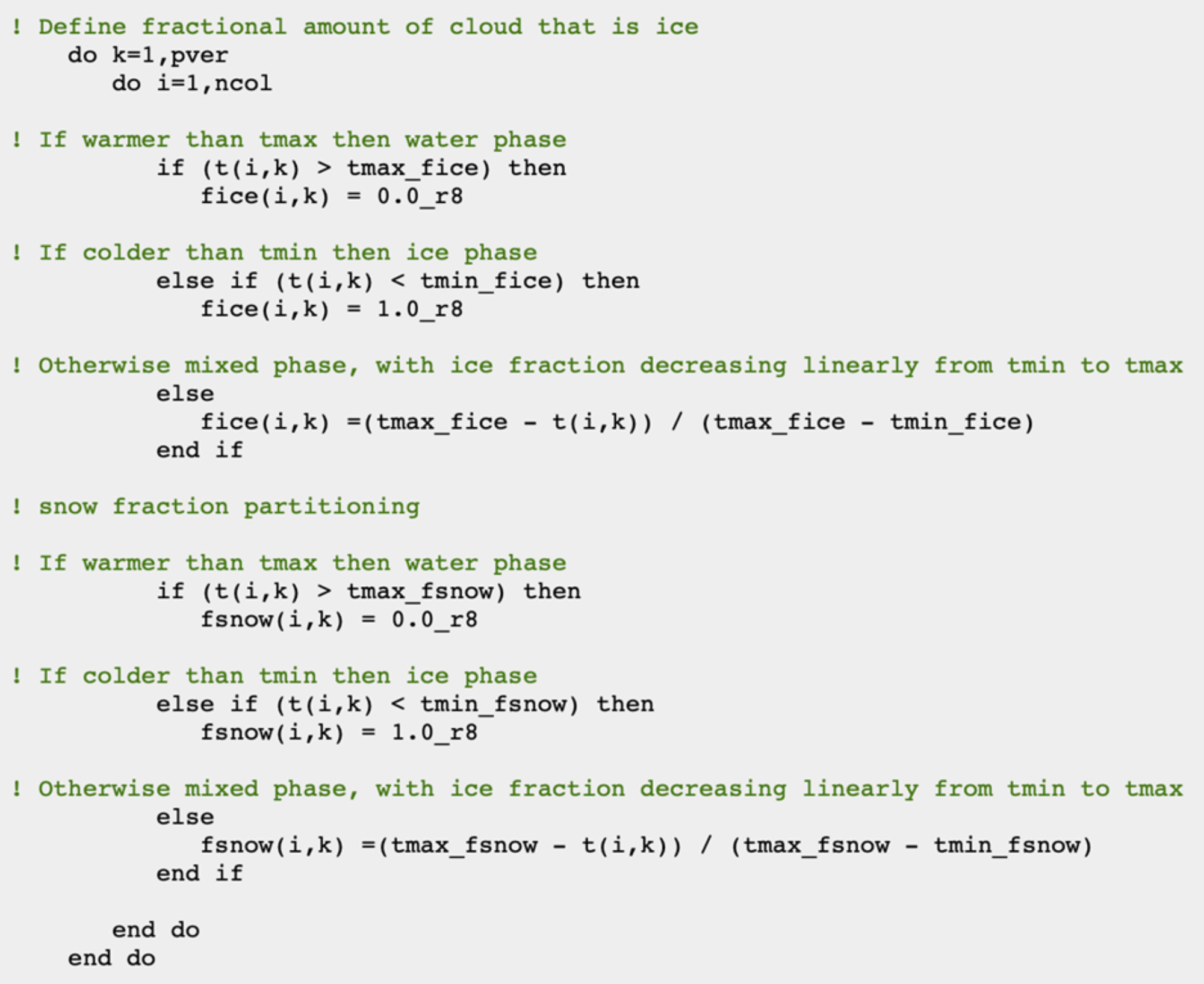
Figure 3: A portion of the FORTRAN code that is used to calculate the split between water, ice, and snow in the Community Earth System Model (CESM) from UCAR. In this example, the model is calculating the fraction of cloud water that is in the ice phase (fice) and the snow phase (fsnow). A modern climate model such as CESM contains well over 1 million lines of code just like this sample. Image by Benjamin Brown-Steiner.
FORTRAN is not taught much anymore, and most climate scientists pick it up as they go. It’s an old language and lacks many of the bells and whistles that modern programming languages include, but it’s stable, reliable, and well-understood. There are a lot of things that you have to do when programming in FORTRAN that you do not have to do in other programming languages and it can be difficult to track down typos, errors, and bugs. But it is not going anywhere, at least anytime soon.

Figure 4: An example of a supercomputer located at the NASA Center for Climate Simulation. Photo by NASA Goddard Space Flight Center (CC BY 2.0 DEED License) via Flickr
This code constructs a framework of functions, routines, sub-routines, sub-models, inputs, outputs, instructions, sub-divisions, and rules that are what makes a climate model “run.” In practice, the running of a climate model is rather boring. You press “enter” and initiate a specific sequence of events, either on a computer in front of you or, more likely, a supercomputer (Figure 4) hosted in some other location, and you wait. Most modelers want to have a file that outputs what the model is doing – often called a “log” – and what is put into this log must be specified before you start the model “run.” If the model is set to run for 100 years, the modeler might want to see some diagnostic output in the log at the end of every simulated month. Experienced modelers can watch this constant stream of model output and gain a sense of what the model is doing. If something is going wrong – say some parameter or variable has skewed away from realistic values, or perhaps some model component is not changing when it should be changing, or changing when it should not be changing – you can track progress. If things go horribly wrong the model will crash and you’ll see this stated in the log. If things go right, the model run will ultimately finish, and you’ll see something in the log along the lines of “Model run successfully completed.”
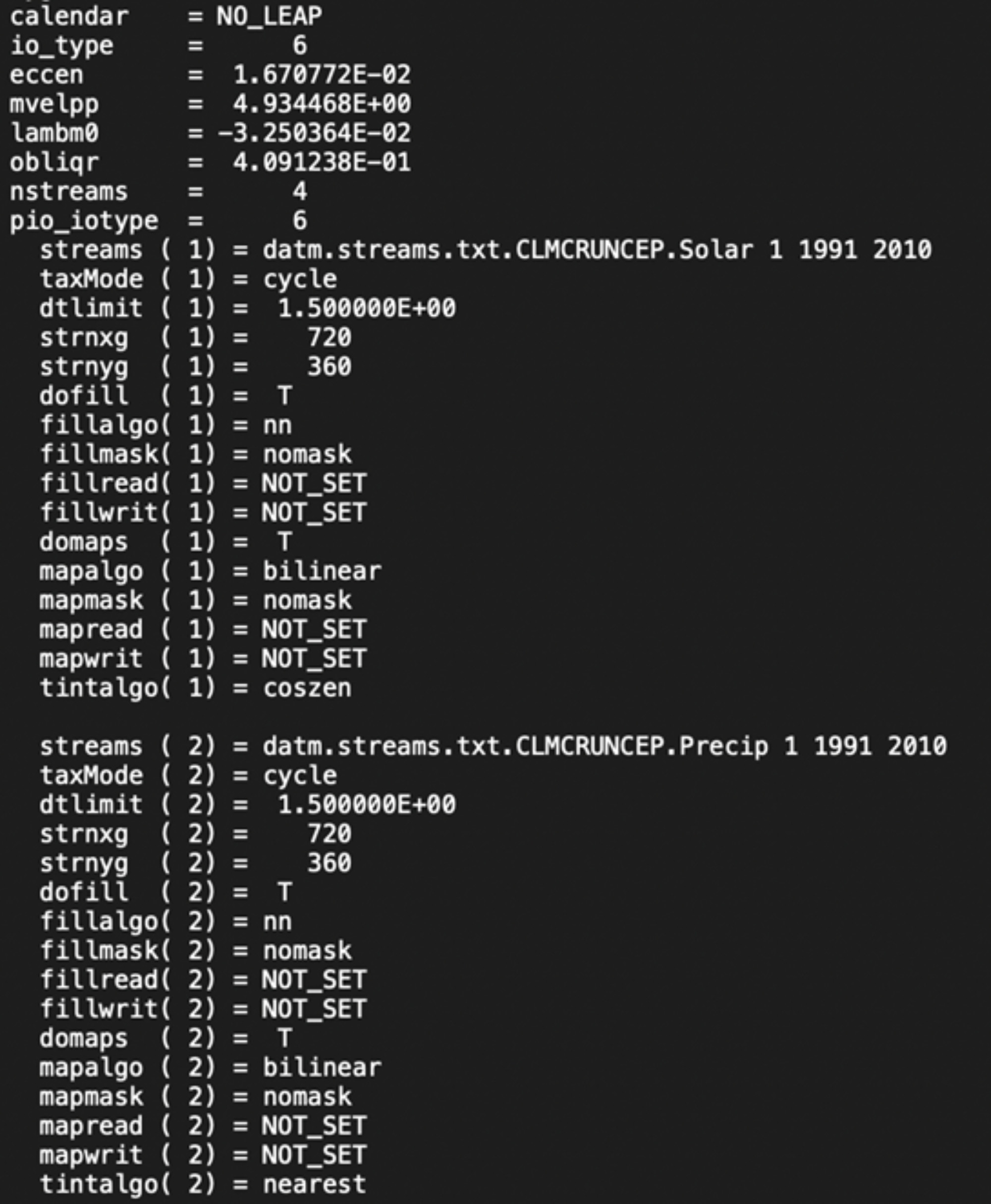
Figure 5: An example of climate model output that is written in a log file. In this example, we can see that the model is running a “NO_LEAP” calendar, which means it simply skips any February 29th during leap years as they make year-to-year comparisons difficult. We can also see that this model is reading input files: solar radiation “Solar” and precipitation “Precip” data between 1991 and 2010. Most of the time these outputs are ignored by researchers, but if something goes wrong or a researcher needs to understand what the model did, the log file can provide clues. Image by Benjamin Brown-Steiner.
However, that message doesn’t necessarily mean that everything ran correctly. It just means that the model did not break. For example, if you coded incorrectly some part of the model such that values did not update as the model ran – say you made a mistake and forgot to include greenhouse gas warming updates to surface temperatures – the model will run and finish fine. Only when you look at the output would you notice that surface temperatures stayed the same. You’d then have to go back and identify your error, correct it, and run the model again. This cycle of code-run-check-repeat is the “meat-and-potatoes” of a climate modeler’s day-to-day experience. Because mistakes and errors can so easily find their way into the climate model code, and because it can be so tricky to identify them, many climate modelers agonize over their model output – not trusting it until it’s been checked and double checked and verified and validated and then triple checked – the climate modeling process can take a very long time before climate modelers write up and share their results.
Initial and Boundary Conditions
While the model itself is simply code that summarizes our understanding of climate science using math, it can act pretty dumb if left on its own. If human coders don’t specifically tell it to stop running if temperatures reach unrealistic values, or end the simulation if some error or bug has resulted in the output being made up of only zeros, the model will hum along contentedly following the instructions scripted by the code until the allotted run time expires. Thus, one major piece of a climate modeler’s job is to ensure that the input data given to a model are as accurate as possible. Two of the primary types of input files are: initial conditions and boundary conditions.
Initial conditions are used by a climate model only once: right at the beginning of a simulation. The purpose of these initial conditions is simple: provide an accurate best-guess value for what every variable is at every grid cell or grid box (Figure 6, Figure 7, and Figure 8) in the model. The model will then update these values using its internal math, science, and code. In a very simple climate model, say one in which the Earth’s temperature is represented by a single value, this would be called T_earth(0), or “the temperature of the Earth at time zero.” For more complex models, with latitude-longitude grids, ocean representations, atmospheric layers, forest sub-models, and so on, the initial condition data set needs to capture a frozen-in-time snapshot of a best-guess as to the initial state of our simulated planet.
Grid Boxes
Grid boxes are the basic subdivision within climate models where the atmosphere is divided into cubes with sides typically along north-south, east-west, and up-down dimensions. Three dimensional models of oceans and ice also use grid boxes. Grid cells or two-dimensional subdivisions (with sides usually along the north-south and east-west dimensions) are found at some flat boundary such as ground. Every grid box or grid cell has a single number for each variable, such as temperature, CO2 concentration, or wind speed. Adjacent grid cells or grid boxes can influence one another, such as when precipitation falls from high in the atmosphere down through vertical layers and ultimately onto the surface.
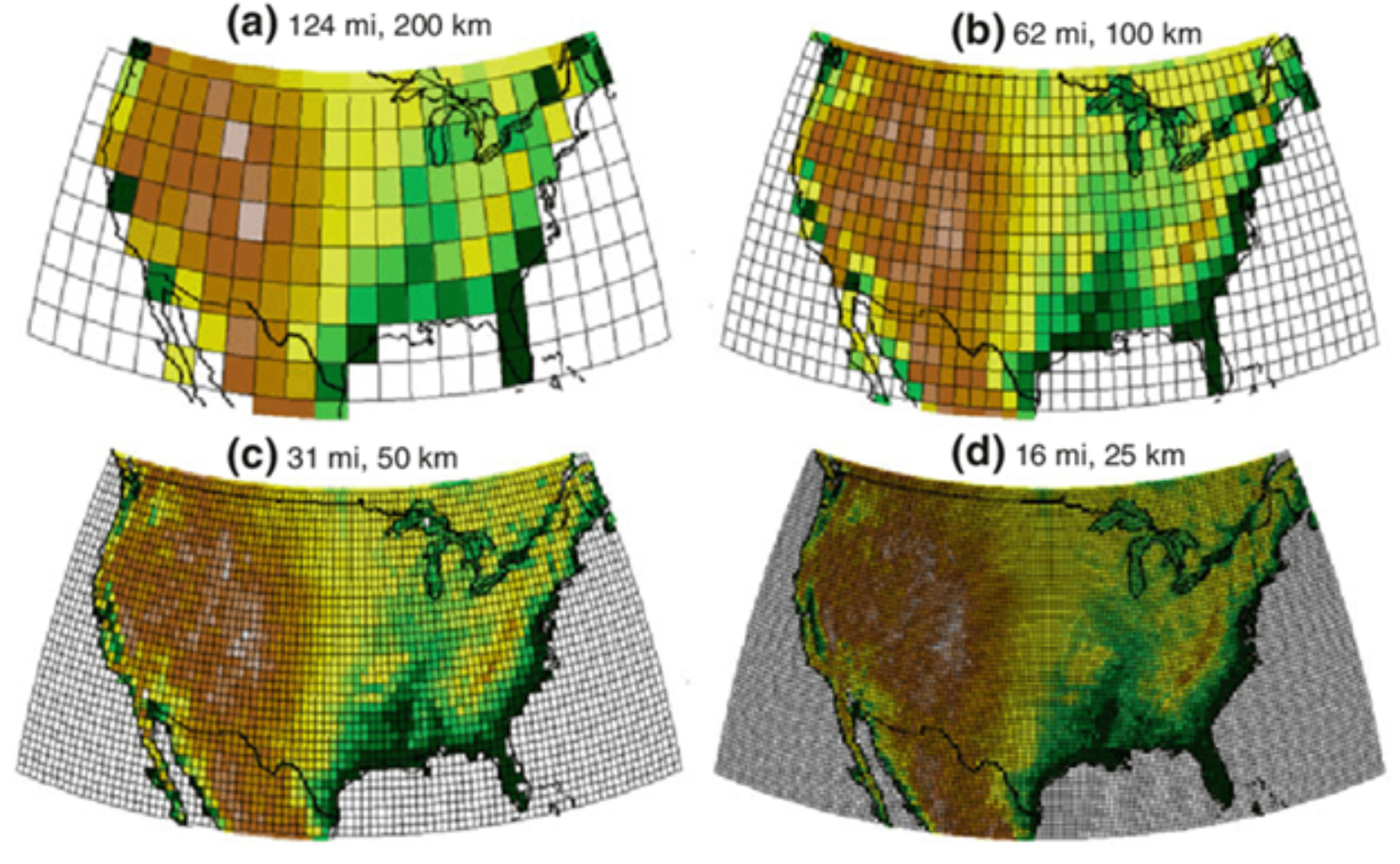
Boundary conditions, on the other hand, serve to provide our model with numerical values representing everything the model does not calculate itself. For instance, climate models do not themselves simulate the cyclical patterns of our sun, and so the changing radiation and brightness of the sun need to be provided to our model as time-evolving boundary conditions. Similarly, most climate models (with the exception of some integrated assessment models, see Climate Emission Scenarios section) do not simulate human emissions internally. Rather they use boundary condition emission file data that include, for instance, how much methane is emitted at every grid cell over the entire Earth’s surface for every time step of the model’s run. Some examples of grids over the U.S. are shown in the following figure, and approximate distances of the grid cell sides are included above each example.
Some climate models can use data from an external “data ocean model” or “data ice model” or “data land model,” so instead of simulating the atmosphere and the ocean and ice and land surfaces, the model runs only the atmospheric model and takes as input boundary conditions from these other sources. These boundary condition files can be assumptions made by researchers or model output from previous ocean or ice or land models.
Needless to say, if the initial conditions or boundary conditions contain errors, the model output will propagate these errors. If there are uncertainties in the initial and boundary conditions, the model is going to incorporate and compound these uncertainties. As a climate modeler, it is important to ensure that your initial condition and boundary condition input files are as accurate and as high-quality as you can get.
Output Data
Climate models do not output everything they calculate while they are running, as this would be an overwhelming amount of data, but they do output a lot of numbers. Climate model output data regularly is measured in the hundreds of gigabytes and sometimes much more. When multiple scenarios are run in order to make comparisons, the output size easily exceeds 1 terabyte (or 1,000 gigabytes). Because of this, climate scientists need to think carefully about what variables they want output and at what time intervals.
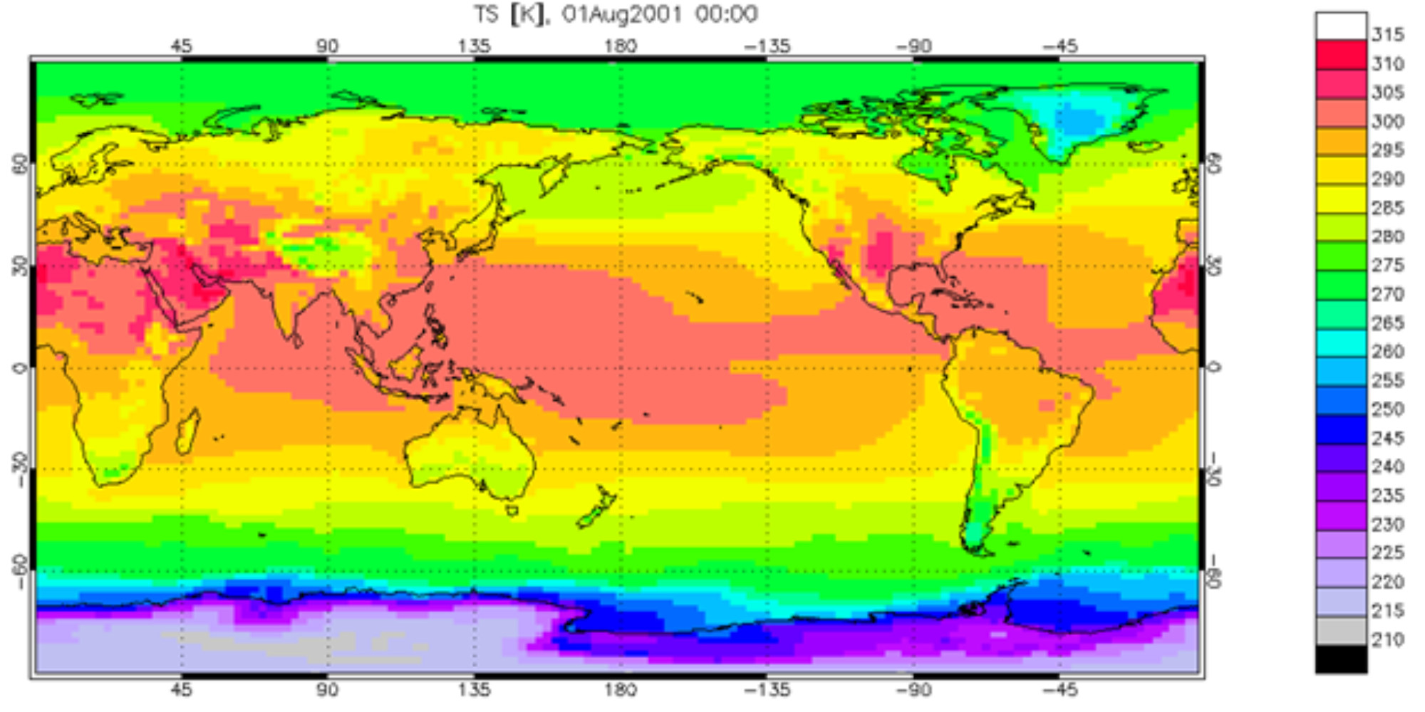
Figure 7: An example of coarsely gridded output data from a climate model simulation. Each grid cell is approximately 2 degrees of latitude or longitude on each side, which translates to roughly 200 kilometers on each side. In this example, global surface temperature data (TS) from August 1, 2001 is shown. Note that these data are plotted in the units of Kelvin, and to convert to Celsius you subtract 273.15 (i.e., Degrees Celsius = Degrees Kelvin – 273.15). Image: Example surface temperature output from the Community Earth System Model (CESM) for a simulation time step of August 1, 2001; screenshot by Benjamin Brown-Steiner.
Most of the output includes gridded output files of all variables of interest – temperatures, radiation fluxes, greenhouse gas concentrations, land, ocean, and ice data, and so on. These output data are often summarized by averaging them across a variety of time intervals. For example, almost all variables of interest are output as monthly averages. Other data are also output at daily or hourly averages, but modelers need to be selective, as output files at fine time intervals can quickly balloon in size to unmanageable proportions.
One final point about output data: not all of it is archived indefinitely. Depending on the community or the purpose of the model run, much of these output data are placed in long-term publicly accessible data archives to be used by other scientists for comparing among models and other purposes. See this link (https://esgf-node.llnl.gov/search/cmip5/) for the fifth iteration of the Coupled Model Intercomparison Project (CMIP5), an example of a climate model output archive available to the public. There are over 50,000 entries in this archive, many of which include multiple files! But output from failed or erroneous model runs and the large amounts of fine time interval data are not usually archived, as they simply are not of interest to a large enough population to make the archiving necessary.
Parameters and Parameterizations
Any complicated machine, such as a sports car or a movie projector, needs to have some set of tuning and adjustment “knobs” for the operator to turn and adjust certain machine components to make sure everything runs smoothly. In a sports car these knobs could be timing belts or fuel flow systems. In a movie projector, these knobs could be color adjustments or a focus lever. In a climate model these knobs are known as parameters and parametrizations.
Parameters are numerical values that can change over time or are set in stone as constants. For instance, the amount of solar radiation entering the Earth’s atmosphere is a time-varying parameter usually set as a boundary condition. An example of a constant parameter is gravity at the Earth’s surface. These parameters tend to sit hidden with the model’s code, math, and science and are typically seen as model inputs rather than model outputs. Parameterizations are relationships between variables and/or parameters that describe known or assumed relationships. If the temperature rises by 2˚ Celsius, how much more water vapor can this parcel of air hold? If solar radiation decreases by 0.1 W/m2, how much colder does the land surface get during the next time step?
Both parameters and parameterizations are contained within the model code and based on math and science principles, but they are often coded in a way that allows climate modelers to access them and change them if needed. This accessing and changing is often referred to as “tuning,” and tuning a climate model can sometimes be as much of an art as it is a science.
For instance, say you run your climate model under an increasing greenhouse gas scenario and, upon examining the output, you note that over time glaciers have covered the entire planet. You could say, “Oh, no! That’s not realistic! There must be something wrong with the ice model!” You could then look back at the model code and, usually after some searching, find a parameter or a parameterization that you suspect caused this error. Perhaps you accidentally made the glacier ice relationship to temperature positive (meaning the higher the temperature the more ice you have) rather than negative (meaning the higher the temperatures the less ice you have). You could adjust this relationship and re-run your model.
Sometimes this iterative process is straightforward: you recognize an error, and you correct it. Sometimes it is anything but straightforward. As we don’t have measurements of every climate variable of interest at every location on Earth, climate scientists need to make a lot of assumptions to fill in the gaps in our observational record. Additionally, our scientific understanding of the climate system is imperfect and contains a lot of best-guesses and assumptions. For instance, we don’t know precisely how quickly a grassy field will lose moisture if the temperature increases and the wind decreases at a given time and location. So, we make our best guestimate, based on physics, chemistry, and what we know about other situations.
Climate scientists know that a climate model contains assumptions and guesses, so when they look at model output and compare to real-world observations and the two do not agree, these scientists return to their model and all the parameters, parameterizations, guesses, and assumptions, and tweak them. Maybe they assumed the ocean surface was too warm during this model run, or that the parameterization that related soil evaporation to wind speed and air temperature was off. One major challenge of climate modeling is the iterative work of testing and refining your model by matching it to a wide set of existing observations and adjusting and tuning parameters and parameterizations.
One pitfall climate scientists can make is hyper-focusing on only one set of model-observation comparisons. Say we have a meteorological station that we trust located in New York State, and we spend time adjusting model parameters and parameterizations until we get the model temperature for New York State to exactly match the observations from the meteorological station. What you have likely done is “overfit” your model to the New York State observations, and while you may have an excellent model-observation match for New York State, it is very likely that you have achieved this match by sacrificing model performance in other locations. There’s a balancing act in which your goal is to get the best possible model-observation matches at the most possible locations.
Climate modeling, as with all modeling, can be a constant balance between overfitting and underfitting and of tuning and adjusting to get the best-possible agreement between model output and all available observations. This process ultimately leads to the final component of model evaluation.
Model Verification and Validation
Finishing a model simulation is not the end of the job for climate scientists – not by a long shot. Once the output data are available, a tremendous amount of effort is needed to compare the data to observations or other climate models, to triple check that individual model components worked the way they were designed to work, and to summarize the massive amount of information in ways that scientists and the public can easily understand. The actual output data is simply a long list of numbers. A long list. This data needs to be interpreted or “post-processed.” Here are a few examples of the types of post-processing that occurs.
Verification
Verification is when model output data is compared to some benchmark established ahead of time to check to make sure everything is working the way it is supposed to work. Think of this largely as a “sanity check.” For instance, you may want to make sure that the methane emitted from the land model was correctly taken in by the atmosphere model, and checking the input and output files of these models for differences is essentially a diagnostic tool to verify that the individual parts are connected properly. Verification is often hard coded into the model run, and can even be coded in such a way that some pre-established diagnostic can end the model run early if a variable diverges from expectations. Think of a kill-switch added to some complicated engine or motor to prevent damage.
Validation
Although validation may seem synonymous with verification, in the modeling community they have very different meanings. Validation is the process by which model output is compared to real world observations or other forms of trusted data sets. While verification can be thought of as an internal check of model performance, validation is more of an external check and, more importantly, an assessment of truth.
It is important to set aside validation datasets in a way that their “real world truth” is not incorporated in the model code, as these validation datasets are the ultimate assessment tool that is used to convince other scientists, and the public, that the model is a good model (that is, accurate enough to be useful). These datasets can be historical observational data averaged over large areas or they can be datasets at specific places or times, and these model-observation comparisons are most often the figures that the public sees. You may have seen figures that show historical model performance compared to historical temperature measurements and model projections of possible future temperatures. For example, a tool called The Climate Explorer lets you explore a wide variety of climate model output for different U.S. cities under different potential future scenarios. A screenshot of what this looks like is included below.
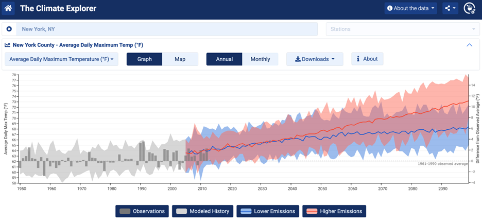
Figure 11: An example of an interactive website that lets you explore various climate model output. In this example, historical and projected future temperatures for New York City are plotted for every year between 1950 and 2100. The grey bar chart shows observations while the lighter grey shading shows the range of model estimates. The red and blue shading represents the range in multiple model predictions of annual temperatures under a high (red) and low (blue) greenhouse gas emission scenarios, while the red and blue lines represent the model average estimates. Image from The Climate Explorer.
Again, the amount of output data produced by climate models is enormous and needs to be checked against a wide variety of real-world datasets. This website looks at maps and time series of climate variables, sea levels, weather data, and extreme temperature or precipitation thresholds, all of which serve as checks of the model performance. These checks ensure that climate models represent the real world as closely as possible, which enhances our confidence that they can accurately estimate future conditions under possible emission scenarios. When new data is produced, from new present-day observations or reconstructions of past temperatures from tree rings, for example, the models are rechecked. When they diverge from observations, scientists work hard to update the model parameters and code. In this way, climate models are constantly improving.